Johns Hopkins Data Science Capstone: Building a SwiftKey Word Predictor in R

This is a look back at one of the more satisfying projects from my Johns Hopkins Data Science Certification on Coursera — the capstone. The assignment was to take a massive corpus of Twitter text provided by SwiftKey and build a word prediction app. Simple enough on paper. In practice, it took a few rounds of iteration before everything clicked into place.

The Dataset

The raw material was a large collection of English-language Twitter posts, blog entries, and news text bundled up by SwiftKey for the course. The corpus was noisy in all the ways you'd expect from internet text — abbreviations, slang, typos, mixed case — which made the preprocessing phase non-trivial. The data was downloaded from the course-provided archive and then cleaned, tokenized, and filtered before any modeling began.

Going Beyond Next-Word Prediction

The standard approach for the capstone was to predict the single most likely next word given what a user had typed. That works, and most of my classmates went that route. But a single-word suggestion feels sparse on a full browser window. I decided to use the entire screen real estate and surface a ranked set of multi-word continuations — essentially letting the model complete a phrase rather than just append one token.

The key insight is that you can chain single-step predictions: take the top prediction, append it, then predict again from the new context. Do that a few times and you have a plausible short completion. The Markov assumption — that the next word depends only on the last n words — keeps this tractable.

N-Grams and the Markov Chain Lookup

The backbone of the predictor is a set of frequency tables built from the corpus. I generated bigrams, trigrams, and 4-grams (n = 2, 3, 4) and stored the counts. At prediction time the app does a backoff lookup: try the 4-gram table first for the best context match, fall back to trigrams if there's no hit, then bigrams, then a unigram fallback.

# Simplified backoff lookup
predict_next <- function(input_words, ngram_tables) {
  for (n in c(4, 3, 2)) {
    context <- tail(input_words, n - 1)
    key     <- paste(context, collapse = " ")
    hits    <- ngram_tables[[n]][prefix == key]
    if (nrow(hits) > 0) return(hits[order(-count)][1:min(5, .N)])
  }
  ngram_tables[[1]][order(-count)][1:5]  # unigram fallback
}

To keep startup time reasonable, the final tables were serialized to an .rds file. Loading a pre-built .rds is dramatically faster than rebuilding the n-gram counts from scratch every time the Shiny app initializes.

The Shiny App

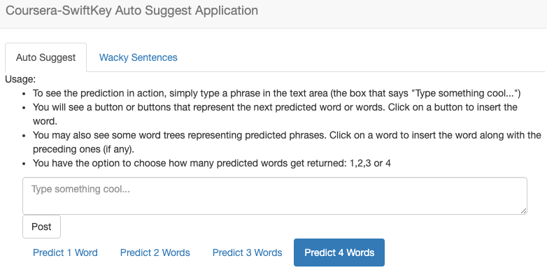
The front end is an R Shiny app. The user types into a text input and the reactive pipeline fires on each keystroke, running the backoff predictor and populating a grid of suggestion buttons across the screen. Clicking any suggestion appends it to the input and triggers a new prediction round — so the user can keep tapping to build up a sentence.

Getting the layout to actually fill the viewport took more CSS wrangling than the NLP did. Shiny's default fluid layout wants to stack things vertically, so I overrode a fair amount of the Bootstrap defaults to get the suggestion buttons to spread out horizontally and use the available width.

What I'd Do Differently

Looking back, a few things stand out:

• Kneser-Ney smoothing would have been a meaningful accuracy upgrade over the raw count-based backoff. I used simple additive (Laplace) smoothing at the time.
• The 4-gram table got large enough to be awkward. Pruning low-frequency entries more aggressively would have cut the .rds file size considerably without hurting prediction quality much.
• A proper train/validation/test split would have made the perplexity numbers more meaningful. I evaluated on a held-out slice of the same corpus, which wasn't quite the same thing.

But the app worked, the predictions were reasonable, and more importantly — it actually felt good to use. Sometimes that's the most honest measure of a project.